[Wang_Bovik_Sheikh_Simoncelli_2004]

Image Quality Assessment: From Error Visibility to Structural Similarity

Resumen:

The main idea in this paper is that human visual perception is built to understand a scene based on its structure suggesting that this structural information is the key component of visual quality. A good way to measure image quality, then, is to quantify the degradation in the structure within a distorted image versus an original.

This is a change in the fundamental assumption from past image quality work. Previous approaches measure perceptual image quality assuming that image intensity is the key component of visual quality. These methods often measure intensity error and then penalize these errors according to visibility.

To get started, let's go over some definitions of commonly used “image quality” terms and abbreviations.

• image quality : a field of study with goals of quantifying subjective human-perceived visual quality and developing objective measures that accurately predict subjective quality
• subjective image quality : human-perceived visual quality, often measured for a group of test subjects and reported as a mean opinion score (MOS)
• objective image quality : quantitative measures that can accurately predict subjective image quality
• full-reference : the complete undistorted original image is available
• no-reference or blind : only the distorted image is available
• reduced-reference : partial information (extracted features) about the original image is available
• MSE : mean squared error, the average of squared pixel intensity differences
• PSNR : peak signal-to-noise ratio s

Error-Sensitivity Approach

The assumption here is that the perceived distortion is directly related to the error signal. These approaches apply a sequence of steps consisting of: preprocessing to scale/align and account for human color perception, CSF (contract sensitivity function) filtering to account for human spacial and temporal frequency response, channel decomposition into temporal and spacial subbands, error normalization according to a perceptual masking model, and error pooling to weight errors and come up with a single quality number.

Some common problems with these approaches have been emphasized in this paper, including:

• the quality definition problem : it's not clear that error visibility corresponds well with image quality
• the supra-threshold problem : most perceptual studies have been evaluated with small errors, where the error is producing a JND (just noticeable difference) and therefore, the studies don't account for large errors very well
• the natural image complexity problem : the images used to develop perceptual threshold are very simple compared to natural images
• the cognitive interaction problem : foveation (where a person is likely to look in an image) and cognation of the image also leads to variable image quality perception

Structural Similarity Approach

The goal of the new approach is to “find a more direct way to compare the structures of the reference and the distorted signals.” The assumption is humans extract structural information from images — not pixel intensities.

An image quality metric based on structural similarity can overcome many of the problems associated with the error-sensitivity method. The SSIM index is one specific implementation of a structural similarity approach — it is not the only possible architecture that uses the structural similarity paradigm, but it is interesting as a first example of structural similarity's utility.

SSIM: An Example Structural Approach

Algorithm Description

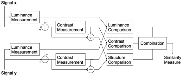
The figure above shows a proposed image quality measurement system that compares registered images x and y . The similarity measure SSIM( x , y ) is a function of luminance l ( x , y ), contrast c ( x , y ), and structure s ( x , y ). Also, it is necessary to include three constants ( C1 , C2 , and C3 ) to prevent unstable results when the denominators approach zero.

The average intensity (ux and uy) is used to define the luminance function

l(x,y) = (2*ux*uy + C1) / (ux^2 + uy^2 + C1) .

The standard deviation (sx and sy) is used to define the contrast function

c(x,y) = (2*sx*sy + C2) / (sx^2 + sy^2 + C2) .

The correlation (sxy) after removing the mean and normalizing by the standard deviation is used to represent structural similarity:

s(x,y) = (sxy + C3) / (sx*xy + C3) .

Finally, the similarity is computed as a combination of the luminance, chrominance, and correlation in a general form

SSIM(x,y) = l(x,y)^a * c(x,y)^b * s(x,y)^g

where a > 0, b > 0, and g > 0 are parameters that determine the relative weighting of each term.

For the specific implementation in this paper, SSIM is simplified by choosing a = b = g = 1 and C3 = C2/2, giving

SSIM(x,y) = ((2*ux*uy+C1)*(2*sxy+C2) ) / (ux^2+uy^2+C1)*(sx^2+sy^2+C2)

Local image statistics are measured in a weighted 11x11 circular window around each pixel to generate SSIM for each pixel. A few other numbers are needed to fully define the parameters C1 and C2 . The dynamic range of the pixels is defined as L (255 for 8-bit grayscale). Then, C1 and C2 are given as functions of L and some small constants K1 << 1 and K2 << 1.

C1 = (K1*L)^2
C2 = (K2*L)^2

In the paper, the author uses these settings: K1 = 0.01; K2 = 0.03. A single number representing overall image quality is computed by averaging the SSIM values to give a mean:

MSSIM(X,Y) = 1/M * sum( SSIM(:) ) .

Test Results

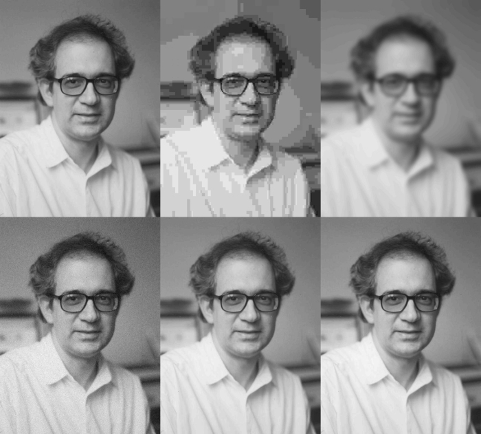
Using the example MATLAB implementation referenced in the paper, I compared MSSIM with mean-squared error (MSE) for a few images. The following figure shows the test images I used.

From left-to-right starting across the top row, these images are 1. the original version 2. jpeg-compressed 3. blurred 4. added gaussian white noise 5. mean-shifted 6. contrast-stretched

All of these versions were created to give an equal mean-squared error (MSE) of 60 — this clearly demonstrates that MSE does not correlate with perceived quality. It is clear that the image quality of 2 and 3 is much worse that the others. Let's see if MSSIM works better.

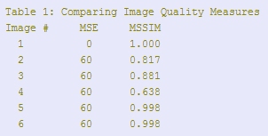
Structural similarity accurately predicts the high quality of images 5 and 6, the mean and contrast-shifted images.

It is interesting to discuss the results from image 4, the one with gaussian white noise added. MSSIM is the lowest for this image, contradicting my expectation that image 4 has a perceptual image quality somewhere between the worst images (2 and 3) and the best images (5 and 6). I wonder why this result didn't match my expectations …

Sumario obtenido de http://dailyburrito.com/blog/image%20processing

Bibliografía disponible:

[]

[]